1.Summary

In Winter 2024, I focused on evaluating and developing several machine learning models to convert images into stroke-based representations. This work was a continuation of my project with Acrylic Robotics, supported by the CoRoM scholarship. The objective was twofold: first, to explore how images can be made paintable by a robotic arm (this post), and second, to investigate how consistent brush pressure on the canvas can be achieved using a feedback control system (link).

In this post, I share some of my insights and preliminary results from the primary exploration (worked on Painterly, DiffVg, LIVE and FRIDA methods), as I did not continue working on this project after March 2024.

2.Technical Stack

🔧 Key Software & Frameworks:

• PyPainterly (painterly rendering)
• DiffVG (differentiable vector graphics)
• LIVE — Layer-wise Image Vectorization
• FRIDA robot painting framework
• SVG vector graphics pipelines

🤖 Robotic arm platforms:

• Mecademic Meca500

🧠 Methods & Algorithms:

• Image-to-stroke conversion with ML models
• Differentiable rendering & rasterization
• Vector graphics optimization with Bézier curves
• Stroke-based painterly rendering

💻 Languages:

• Python

3.Painterly

A Python implementation of Aaron Hertzmann’s Painterly rendering algorithm for stroke-based image generation is available this repository. The figure below illustrates the architecture of the main code modules in the GitHub repository. The input variables are input image path, radii, output saving path, threshold of similarity, straight or curved lines, spacing between strokes, and debugging.

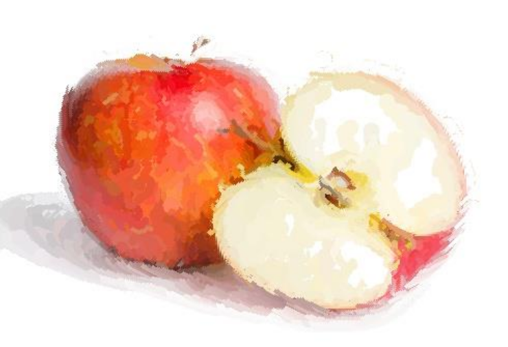
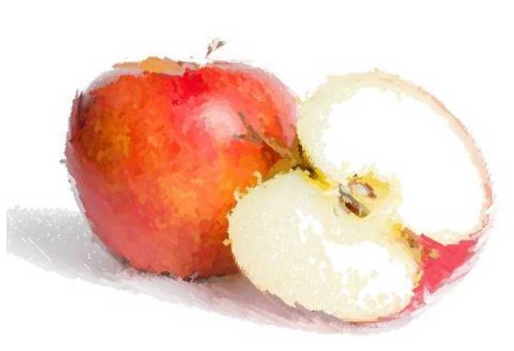
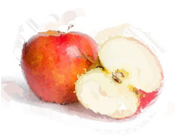
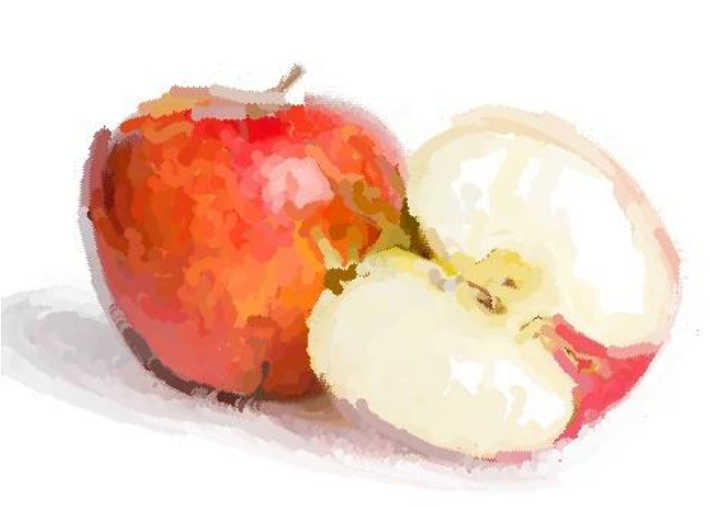
I tested this method using the original image shown below (input image shape: 1200 × 1200 × 3). To reduce computation time and enable faster training, all images were resized to 500 pixels.

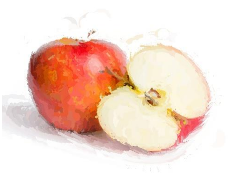
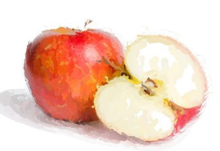
When the approximation threshold T was varied, its effect on the output was relatively minor. For example, the results shown below correspond to T = 100, 50, 20, and 5, respectively, and the visual differences are limited.

T = 100

T = 50

T = 20

T = 5

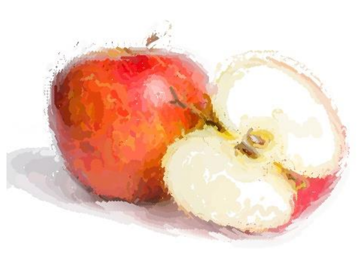
In contrast, brush size had a significant impact on the output quality:

• Size 2: Provides fine details but introduces noticeable gaps.
• Size [8, 4, 2]: A well-balanced combination that produces a decent and visually pleasing result.
• Size 12: Using only a thick brush does not add much value and reduces detail.
• Size [12, 2]: The large gap between brush sizes negatively affects the output quality.
• Size [20, 2]: The gap becomes even more pronounced, and the thick first layer significantly reduces quality.
• Size [20, 12, 8, 4, 2]: Although this is a multi-scale combination, the inclusion of brush size 20 decreases overall quality.

Size 2

Size [8, 4, 2]

Size 12

Size [12, 2]

Size [20, 2]

Size [20, 12, 8, 4, 2]

Overall, the results suggest that overly thick brushes reduce rendering quality. Since I did not test these configurations on a physical robot, it is difficult to determine the optimal brush combination in practice. However, [8, 4, 2] appears to be a promising balance between detail and coverage.

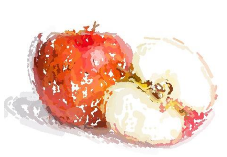
I also experimented with straight-line strokes. The visual outcome is interesting, but it remains unclear whether such strokes are physically paintable with a robotic system. Exploring other curve types could also be valuable. The examples below correspond to [8, 4, 2] and 12, respectively.

[8, 4, 2]

12

Another important parameter is f_g, which directly affects the grid sampling and pixel sweeping process. Its default value is 1. When increased, the output begins to show gaps and incomplete coverage. The figures below illustrate results for f_g = 0.5, 1, 2, and 5, respectively.

f_g = 0.5

f_g = 1.0

f_g = 2.0

f_g = 5.0

Some open questions that remain for further investigation:

• How can radii defined in pixel space be accurately converted into real-world brush thickness? What parameters are required for this conversion?

4.DiggVg

One of the most effective methods that significantly improved image rendering quality was proposed in the paper titled “Differentiable Vector Graphics Rasterization for Editing and Learning.” The authors introduced a differentiable rasterizer for vector graphics that bridges the raster and vector domains through backpropagation. This differentiable rasterization framework enables a wide range of novel vector graphics applications. Detailed information about the paper and its implementation is available at this link.

In this section, I share insights from my evaluation of this method. The main input parameters include: input_image, num_paths, max_width, use_lpips_loss, num_iter, and use_blob. The input image used for testing is the same one described in the previous section.

Effect of num_paths

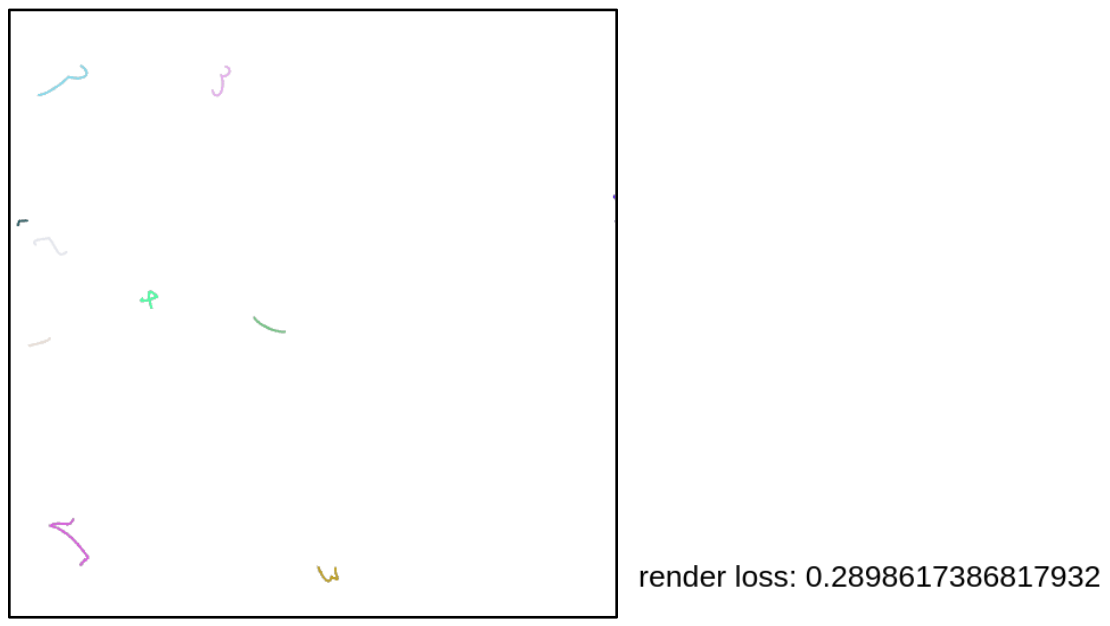
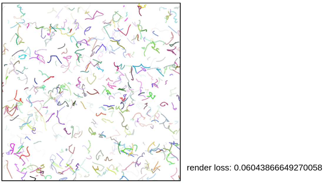
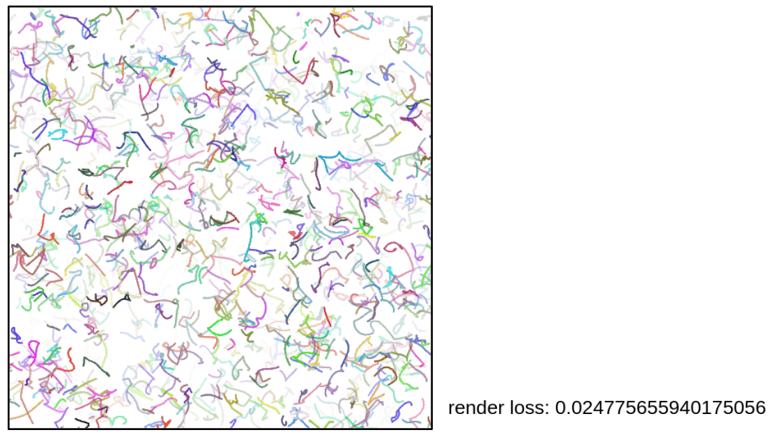
The num_paths parameter directly affects the optimization process and the loss value. I tested three different values (with the same number of iterations): 10, 512, and 1000. After 50 iterations, the corresponding loss values were 0.289, 0.060, 0.024, respectively.

The reason is straightforward: a larger number of initial strokes allows the model to approximate the image more effectively and converge faster. These strokes are initialized on a white canvas. With only 10 initial strokes, for example, convergence becomes very difficult.

Technically, num_paths determines the number of < path > elements in the SVG XML file. The rest of the optimization process updates these paths to minimize the loss. Therefore, this parameter should not be set too low, as it directly limits the model’s expressive capacity.

num_paths = 10

num_paths = 512

num_paths = 1000

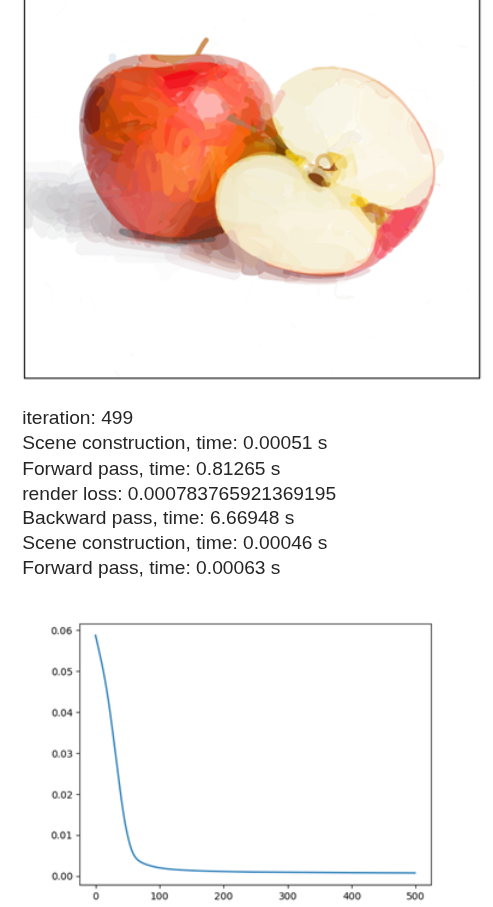
Effect of max_width

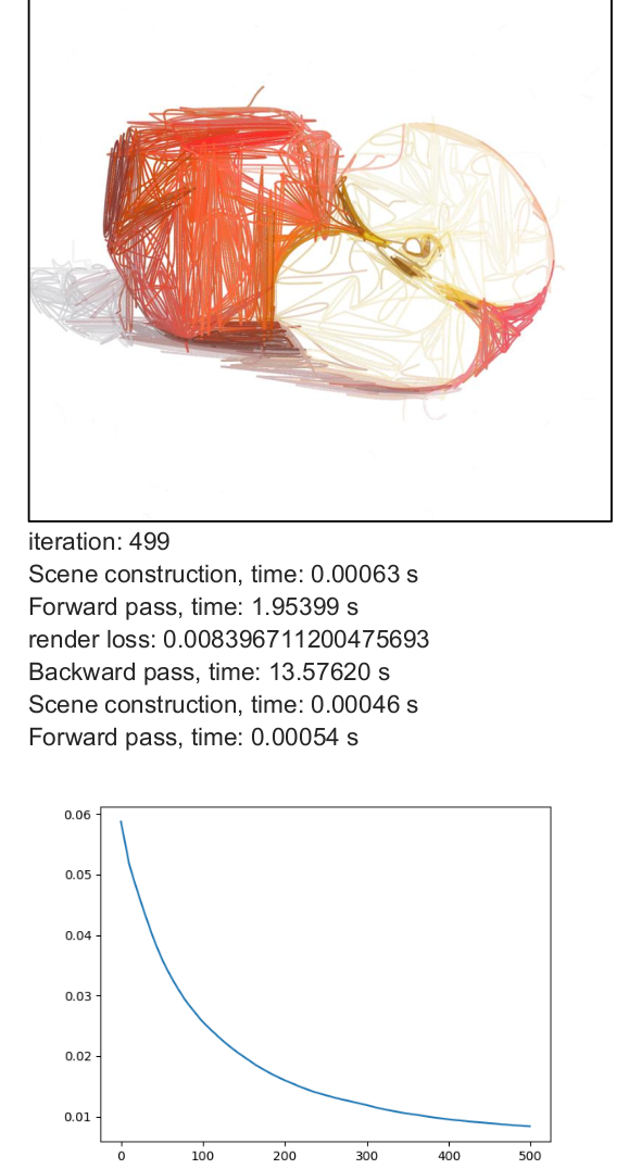
The max_width parameter defines the maximum stroke thickness. The minimum stroke width is 1, and the maximum allowed value is max_width. I evaluated different values of max_width using 500 iterations with num_paths = 512 as a baseline.

Analysis:

• Stroke thickness is treated as a continuous variable between 1 and max_width.
• Increasing thickness generally helps the model converge faster.
• Thicker brushes introduce stronger gradient blending effects in colors.
• By examining the SVG XML files, it becomes clear that the optimization often pushes stroke widths toward the upper bound (max_width).
• This suggests that allowing thicker strokes increases the model’s ability to reduce reconstruction error more quickly.

max_width = 2 (82 min)

max_width = 8 (63 min)

max_width = 20 (62 min)

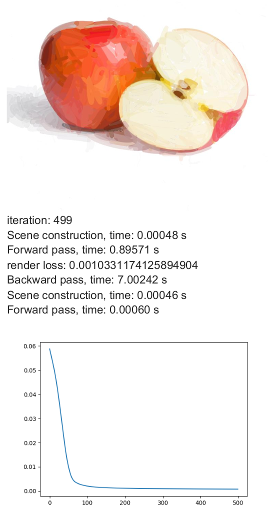
Effect of use_lpips_loss

I also tested the LPIPS loss function using max_width = 8, num_paths = 512, and num_iter = 500. Previous experiments were based on the Mean Squared Error (MSE) loss, whereas this configuration used LPIPS. LPIPS compares deep feature representations in latent space rather than performing direct pixel-wise comparisons.

Analysis:

• The formulation of LPIPS differs significantly from MSE and may require different initialization settings.
• The rendered colors appear more solid and less blended.
• The output is perceptually meaningful but not always pixel-wise close to the original image. -Interestingly, the solid color effect could be advantageous for real robotic painting, where transparency and subtle blending are harder to reproduce.

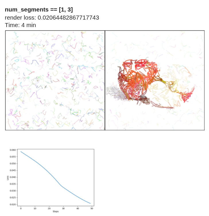
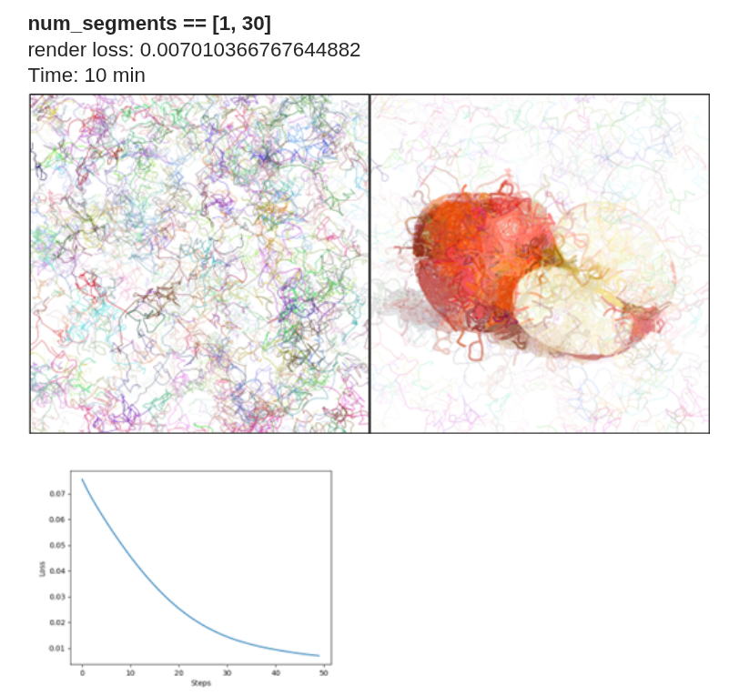
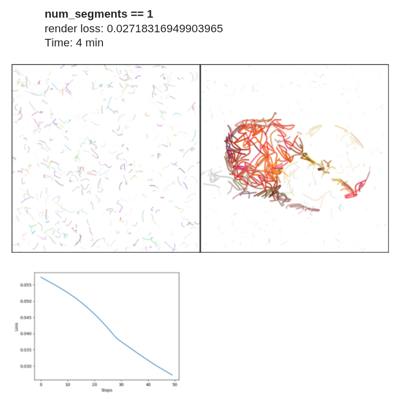
Effect of num_segments

To establish a fixed baseline, I used 50 iterations with max_width = 8 and num_paths = 512. It is important to distinguish between num_paths and num_segments:

• num_paths determines the number of initial strokes.
• num_segments defines the number of Bézier curve segments per stroke.

In the implementation, p0 represents the starting point, and p1, p2, and p3 define a cubic Bézier curve (one segment). When num_segments = 1, each path contains four control points corresponding to a single cubic Bézier curve.

When num_segments = 2, two Bézier curves are generated, typically sharing the same origin. As num_segments increases, the complexity of each stroke increases. For values between 1 and 30, a large number of curves can be generated, significantly increasing stroke density on the canvas Thus, num_segments directly influences stroke flexibility and geometric complexity.

num_segments == [1, 3]

num_segments == [1, 30]

num_segments == 1

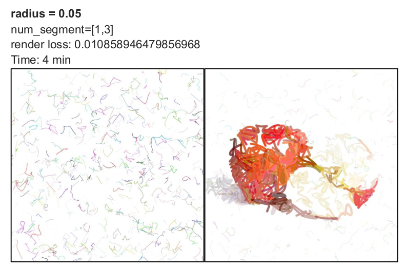
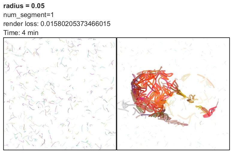
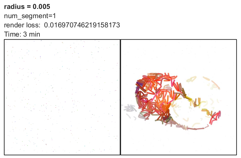
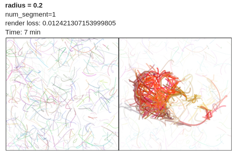
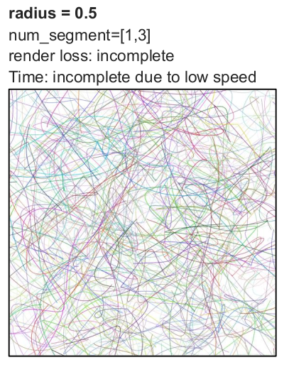
Effect of radius

By default, the radius parameter is set to 0.05. I evaluated its effect using 50 iterations with max_width = 8 and num_paths = 512.

The radius determines how far control points are initialized from the starting point. The formulation follows: x1 = x0 + r(random - 0.5) A similar equation applies to other control points and the y-axis.

Analysis:

• Smaller radius values keep control points close together, resulting in shorter and more compact curves.
• Larger radius values produce more extended and diverse strokes.
• Radius does not directly determine convergence speed but influences rendering complexity.
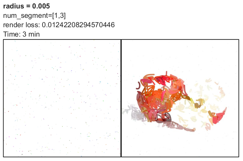
• For a single Bézier curve, testing radius values of 0.005, 0.05, and 0.2 showed slightly lower loss at 0.2.
• For higher iteration counts, larger radius values may converge faster.
• However, increasing radius significantly increases rendering time.
• For very large values (0.5 or 1), the computation became too slow, and I stopped execution.

Overall, radius represents a trade-off between stroke diversity and computational efficiency. Moderate values such as 0.05 or 0.1 may offer a reasonable balance.

Size 2

Size [8, 4, 2]

Size 12

Size [12, 2]

Size [20, 2]

Size [20, 12, 8, 4, 2]

use_blob Differences between if args.use_blob and else:

With use_blob:

• random number is between 3 and 5
• There is a condition for p3: if j<num_segments -1
• Path is closed: is_closed=True
• Since the path is closed, there is a color for filling: fill_color=…

Else:

• random number is between 1, 3
• There is no condition for p3
• Path is not closed: is_closed=False
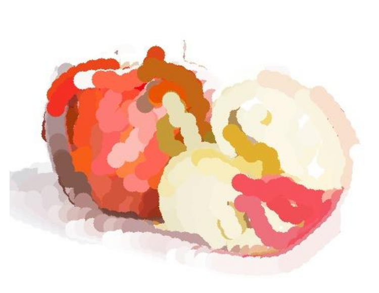
• Since the path is open, there is a color for stroke: fill_color=None, stroke_color=….

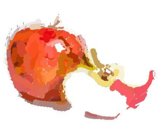
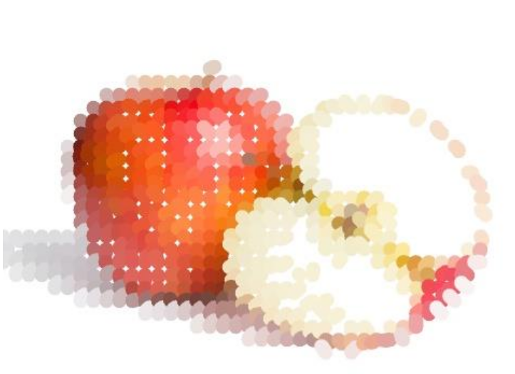
We don’t need this feature because the output is not a stroke (like below image).

5.LIVE

Another promising method is LIVE, which stands for Layer-wise Image Vectorization. This approach converts raster images into SVG representations while preserving image topology. It was introduced in the 2022 paper titled “Towards Layer-wise Image Vectorization.” The paper and implementation are available at this link.

In this section, I share insights from my evaluation of this method. The input image used for testing is the same one described in the previous sections.

Effect of max_path

The max_path parameter directly corresponds to the number of layers (i.e., paths or strokes). To achieve a complete and detailed output, this value must be sufficiently large. If the number of paths is too small, the model lacks the capacity to approximate the image effectively.

max_path: 3

max_path: 10

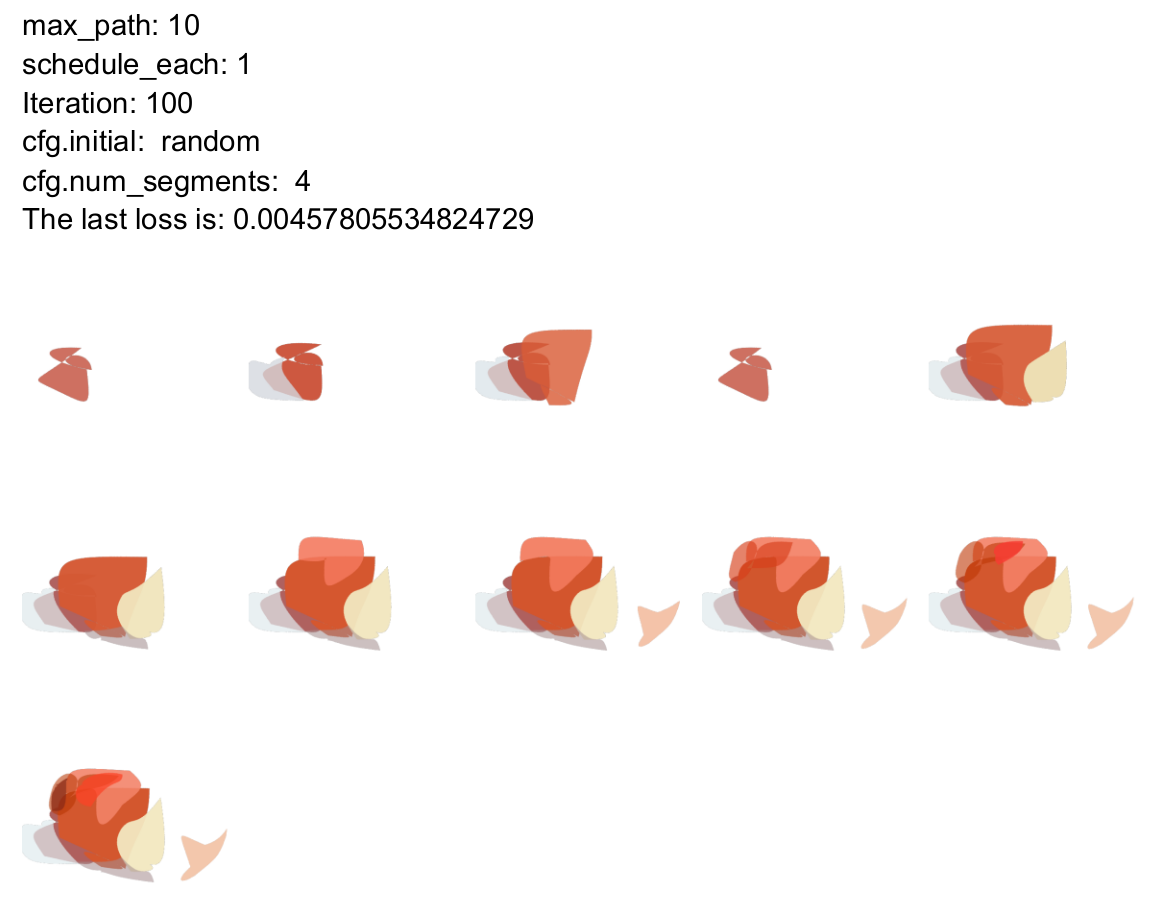
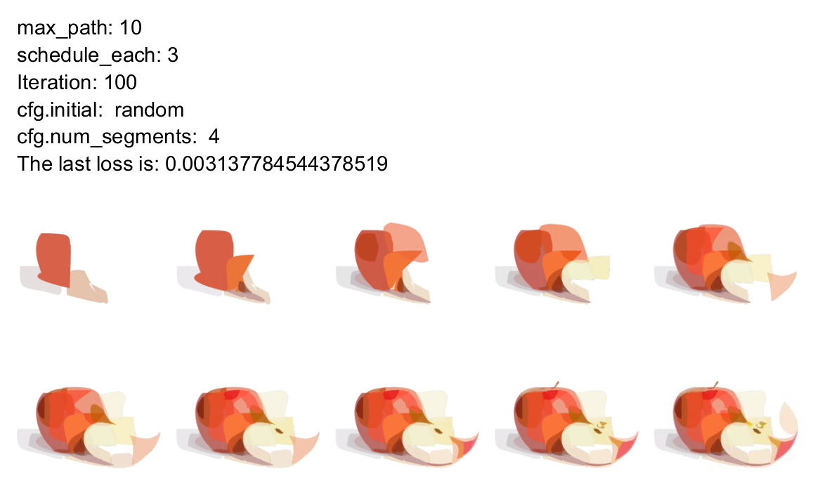
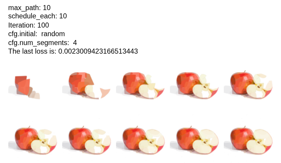
Effect of schedule_each

This parameter determines how many strokes begin optimization at each layer. For example, if schedule_each = 3, three new strokes are initialized and optimized at each step.

Observations:

• Compared to lower values, increasing this parameter reduces the loss value.
• As schedule_each increases, convergence improves.
• A larger number of strokes being optimized per layer allows the model to approximate the image more efficiently.

schedule_each: 3

schedule_each: 10

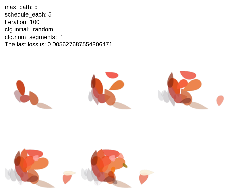
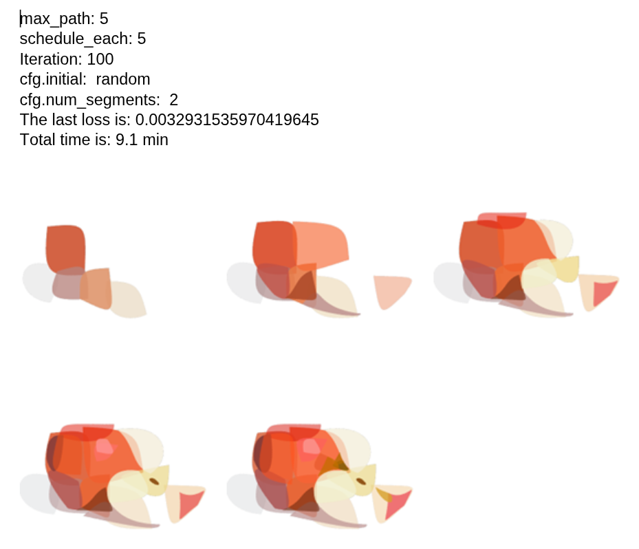
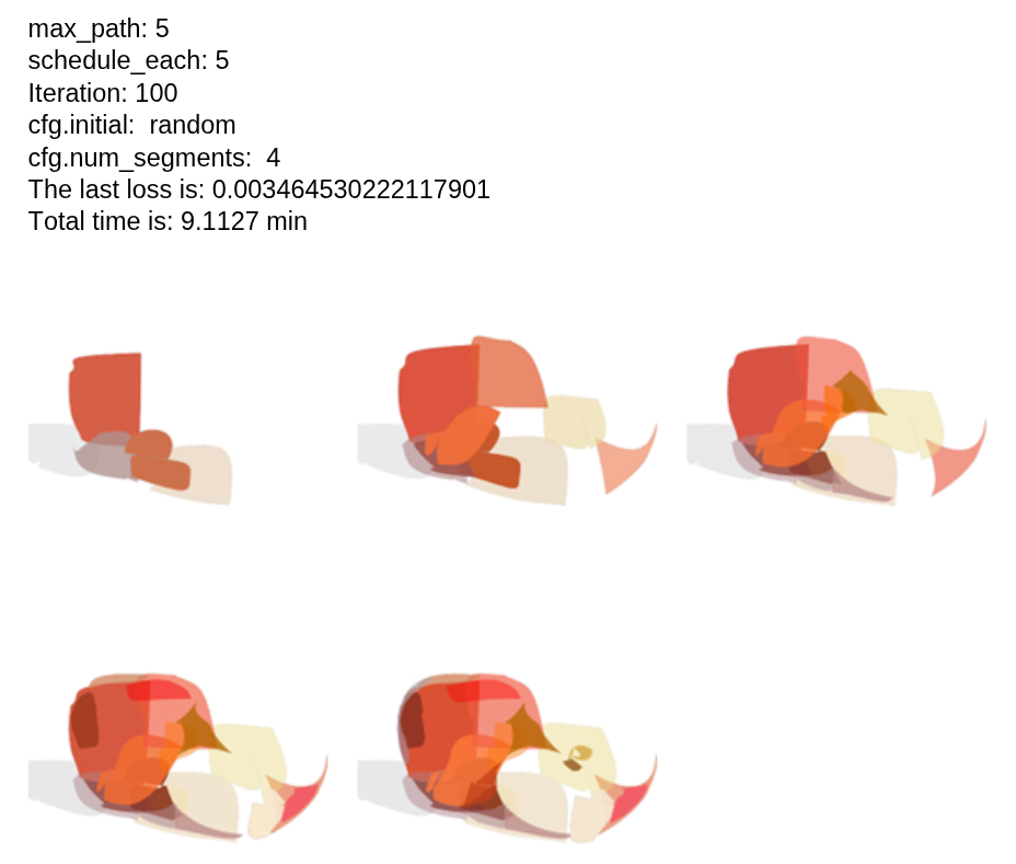
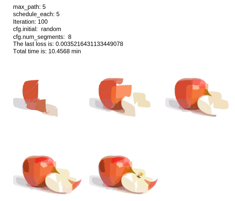
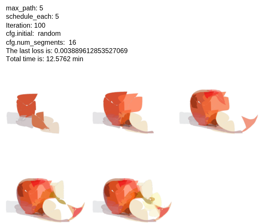
Effect of num_segments

I modified this parameter at initialization and tested it for 100 iterations, with 5 layers and 5 strokes optimized per layer.

Analysis:

• There is no clear or direct relationship between the number of segments and the loss value.
• There is also no consistent relationship between the number of segments and runtime.
• Increasing the number of segments generally improves visual output quality.
• However, the relationship is not monotonic or easily predictable.

In general, num_segments directly influences rendering flexibility and stroke complexity, but its impact on loss and runtime is not straightforward.

num_segments: 1

num_segments: 2

num_segments: 4

num_segments: 8

num_segments: 16

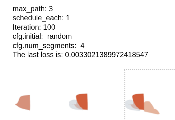
Effect of initial Parameter

By default, the initialization is set to random. I modified it to circle for comparison.

Analysis:

• Comparing random (with 4 segments) and circle initialization shows very similar loss values and runtime.
• The visual outputs are also quite similar.
• There is no significant advantage in using circular initialization over random.

The second image below illustrates this comparison (left: random, right: circle).

Background Optimization (bg Parameter)

To activate background optimization, the bg parameter in the YAML configuration file must be set to True (bg: True).

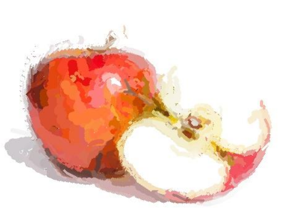
Scenario 1: Apple Image (Solid Background)

• Parameters: Iterations = 100, max_path = 5, schedule = 5

• Analysis:

  • When bg=True, the model attempts to optimize the background in addition to the foreground.
  • This increases runtime and produces a more colorful background.
  • Without background optimization (bg=False), the model converges faster under the same parameters.
  • The difference is particularly visible in the half-apple example.

Scenario 2: Image Without Solid Background

• Parameters: Iterations = 100, max_path = 5, schedule = 30
• Analysis:
  • Without background optimization, the rendering appears more complete.
  • With limited iterations and paths, the difference is subtle.
  • Based on these tests, background optimization does not appear necessary for this application.

Comparison of Initialization Types: random, naive, sparse

I compared the three available initialization strategies: random, naive, and sparse.

Observations:

• Loss values and runtime comparisons are presented below.
• Although the random initialization achieved slightly lower loss values, the sparse initialization produced the best visual output in my evaluation.

After conducting several simulation tests, a number of open questions remain. The following points arose before performing a detailed review of the implementation code:

• Is it possible to develop a clear and systematic model for determining the optimal combination of key parameters for each input image?
• Since this method appears to be slower than DiffVG, what is its main practical advantage? The paper primarily demonstrates results on emoji-style images, which may not be sufficient to validate its effectiveness on more complex images.
• Is it possible to adapt this method to use stroke-based curves instead of closed curves?
• In terms of solid color rendering, does this method perform better than DiffVG, particularly when opaque strokes are required?

Comparison: DiffVG vs. LIVE

After evaluating both methods, I conducted a qualitative and quantitative comparison between DiffVG and LIVE under different configurations.

• Achieving a reasonable rendered image with LIVE generally required fewer strokes compared to DiffVG. For example, in DiffVG, using only 10 paths (strokes) made convergence difficult and time-consuming, while 512 paths provided stable and acceptable results. In contrast, LIVE was able to reach a visually decent output with approximately 30 strokes in total (e.g., 10 paths with a schedule of 3). It is important to note that LIVE uses closed Bézier curves rather than open stroke curves. This structural difference likely contributes to its faster convergence in terms of stroke efficiency.

• Since the stroke representations differ significantly between the two methods, directly comparing them in terms of the number of segments is not straightforward. Additionally, the internal modeling of strokes in LIVE is less transparent and was not fully clear from the implementation.

• I tested LIVE with the following parameters:

  • max_path = 25, schedule_each = 10, num_iter = 200. This configuration resulted in 25 layers and a total of 250 strokes.
  • For DiffVG, I used: num_paths = 512, num_iter = 500, max_width = 20.
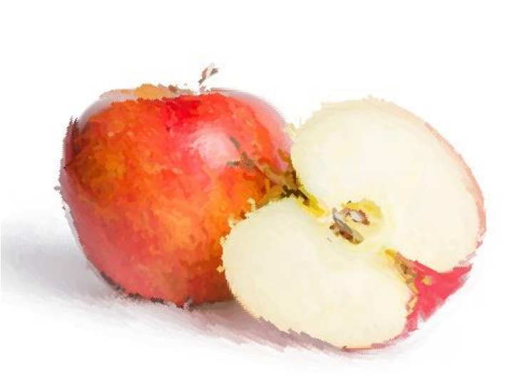
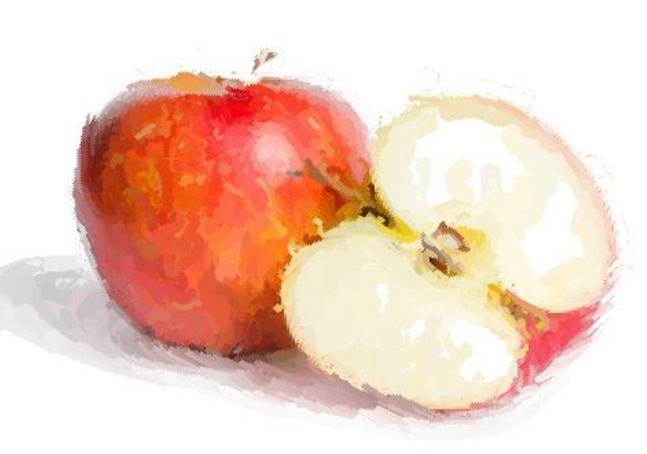
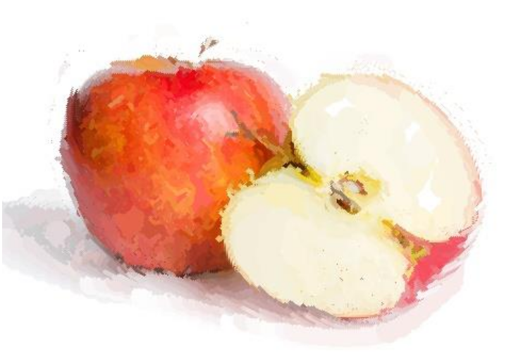
  • Below is a side-by-side qualitative comparison (right: LIVE, left: DiffVG).

• Observations
  • Visually, LIVE produced better perceptual quality, particularly in shadow regions and smooth transitions.
  • Colors appear more opaque in LIVE, although both methods utilize gradient-based strokes.
  • LIVE achieved comparable visual quality with roughly half the number of strokes and fewer iterations. However, it required longer runtime overall (~155 minutes for LIVE versus ~62 minutes for DiffVG).
  • The difference in stroke modeling (closed Bézier curves in LIVE versus stroke-based curves in DiffVG) should be considered when interpreting these results.
• Although the loss functions differ and are not strictly comparable, the final values were: DiffVG: 0.00078 and LIVE: 0.00185.